Prosthetic Arm Control

Autonomous Robot

Robot End Effector

Mobile Manipulator Control

Physics Simulation

Mobile Manipulator Control

Complete software for motion planning and controll for KUKA's YouBot, simulated in coppeliaSim

Motion Planning
Task Space Control
Kinematics and Odometry

Prosthetic Arm Control

A prosthesis with 1 DOF elbow joint to swing in time with users walking pattern

Zephyr RTOS
Embedded Systems
PID Control

The mechanical design of this arm had been completed by previous researchers (which I will be revamping in future research). So, this project focused almost entirely on writing software to maximize the performance of this design.The prosthetic has a elbow joint with a servo motor inside, controlled as a normal brushed DC motor (not using the servo's position controller). Then, there is a plastic forearm component connected to the motor with the Fillaer E-400 Elbow.Finally, there is an external hardware box. This contains the pcb with the microcontroller (Teensy 4.1) and all other breakout boards such as the IMU (MPU 6050), current sensor (INA 219), motor driver (DRV8871), and voltage regulators.This system was controlled using Zephyr, a Real Time Operating System (RTOS) that can perform scheduling on threads. Zephyr is not entirely supported on the Teensy, however, I have created a guide for building, flashing, and basic use of Zephyr on Teensy on my github. This repository also includes all the code used in this project.

Prosthetic Arm in Bench Testing Rig

The control system used, as described in this diagram, is a doubled nested loop of position and current control. With the potentiometer in the servo motor as a rudimentary encoder and a current sensor, I could create two robust feedback loops to control the arm's position. For both these control loops I used PIDF control, and was able to attain a high degree of precision during bench testing.

Bench Testing Participant Data at 1.1m/s

The results to the left are an output from a bench trial on the prosthetic arm. As you can see, the position controller (plot on the right) is able to follow the prescribed trajectory with some precision. After tuning my controllers during bench testing, my team and I decide to see how the arm would behave during testing on a participant.
Before testing, we wanted to implement a way for the arm to recognize walking from stationary actives. The way that I implemented my own algorithm to detect such activity can be seen below.

Error

Understanding error is key to understanding PID control. Error as defined in this setting is the actual value subtracted from the set point (desired) value. This calculation gives us a quantity to determine how far off the controlled value is from the desired. This value is then manipulated by the coefficients in PID control to produce a new value known as 'u'. This value is then used to make a change in the system and close the control loop. As seen to the right, error can be both positive and negative. The controller deals with both signs, but the way that this value is used may need to be adjusted as is done in this system.

error = setpoint - actual;

Proportional (P) Control

Proportional control is the first term in PID control, and the easiest to understand. To find the proportional term you multiply the error by the proportional term coefficient (often denoted as K_p. This proportional response can be analogized as a spring response with a stiffness k. The higher the stiffness, the stronger the response. So, you can think of proportional response as the direct response to error in your feedback system. As you can see to the right, this output shows a controller which needs a higher K_p value so that it can reach the highest and lowest set point values. Be warned, it is important that your K_p value is not too high as that can result in unwanted oscillations.

P = Kb * error;

Integral (I) Control

The integral response is a way of accounting for error that adds up over time (hence the name). The integral response can be found by multiplying the integrated error (cumulative sum of error multiplied by timestep) by K_i, the integral response coefficient. Integral response is best at accounting for steady state error, that is error which is too small to generate meaningful proportional response but still exists. One important note is that integral response often requires some anti windup mechanism to prevent extreme behavior. For instance, if the error spikes due to a large set point change the integrated error can quickly accumulate or 'windup'. This can generate huge responses from the integral term that are not desired. One way to prevent this is called 'clamping' where you set a maximum and minimum value for the integrated error. This will prevent such behavior to an extent.Another problem integral response can bring is slowing down the controllers response time. If the integrated error quickly saturates in one direction preceding a direction change by the set point, it will need to wind down before generating a response in the opposite direction. This made using integral response in my controller less attractive since I was trying to reduce delay in the controller, which you can see in the final coefficient values I selected. You can see to the right an example of this integrated error induced delay especially while tracking negative steps after accumulating error on the positive steps.

integrated_error += error * dt;
I = Ki * integrated_error;

Derivative (D) Control

Derivative response has a 'slowing' effect on the controller. The differentiated error can be summarized as the change in error over one time step. This is then multiplied by the coefficient K_d which produces a response that is in essence proportional to the rate of change of the error. So, it will produce large response when the error changes and then rapidly decreasing response as the controller corrects for the change in set point.This type of control was important for me since it increases the immediate response to change, which can help offset delay due to the gearbox friction. One important note is that derivative response is highly sensitive to noise and often needs filtering on the error inputs to remain somewhat stable. Additionally, K_d coefficients that are too large can introduce wild oscillations into the system, as seen in the figure to the right.

differentiated_error = Kd * (error - previous_error) / dt;
D = Kd * differentiated_error;

Feed Forward (F) Control

Feed forward control is calculated without error input. Instead, it takes the set point value and scales it with the feed forward coefficient K_ff. Feed forward response is critical in delay prone systems like the prosthetic arm, and helps the controller to predict what the set point will desire next.

F = Kff * setpoint;

Find u and Complete the Feedback Loop!

The final step is to sum all the PIDF components to find u. This is the controller command, and needs to then be transformed into something useful. Referring back to the controller block diagram, the u generated by position control is used as a set point for current control. The u generated by current control is used to generate a PWM value used to drive the prosthetic arm. Then, the resulting change in position is measured by the encoder and the feeback loop is complete!

u = P + I + D + F;

Example of Error

Example of Higher P Required

Example of windup issues (amongst others)

Example of too large K_d coefficient

Results from Successful Bench Testing

With data from an IMU that was a part of the embedded system, I drew upon data only in the direction perpendicular to the ground while the arm was in use. Then, using my own data collected while walking I determined two thresholds. First, a higher threshold that when passed would indicate a step has been taken. Then, a second, lower threshold that must be passed to ensure that the step has 'ended' before another step can be found. The diagram to the right shows how this step detection performs on my walking pattern.The next step after developing this algorithm was to use it to select a arm swing trajectory.

Step Detection Performance

With the help of a participant I tested the position control scheme for a user on a treadmill The most exciting findings were that at faster walking speeds (1.1m/s and 1.3 m/s) we saw some success in following the arm swing trajectories! This was a huge win for the project, where the arm has not successfully run ever during a human trial.This came with a qualification of course. The successful behavior observed was periodic because the arm swing would come in and out of phase with the participants arm swing. This is despite the fact that the data was collected from the same person at the same speed on their other arm. We know that the periodic success is because during this cycle the arm is fighting against the momentum of our participants arm swings sometimes, making it seem like the arm is not moving.Furthermore, when examining trajectories collected during successful arm swings there is a pronounced over shooting in the current control. The momentum resulting from the participants arm swings is propelling the arm and causing 'output' current to be higher than desired. You will also notice that the second mini swing in the arm trajectories is completely omitted.

Arm Swing Trajectory Collected at 1.3 m/s

IMU and Step Detection Collected at 0.7 m/s

As for the step detection and variable arm swing selection algorithm that I created -- it did not perform as expected during testing. The greatest issue occurred when I realized that the footfalls of our participant resulted in different magnitude IMU peaks than my own testing. This might have been because of the different treadmill we were using or her own walking pattern.Additionally, I found that her walking cadence at the speeds we were using was vastly different from what I estimated. Even after making adjustments to the parameters in both these critical steps, the variable speed detection did not work in the end.In the arm swing trajectory plot to the right you can see how the arm comes in and out of phase with the arm swing of the participant. You can also see that the step detetcion algorithm was successful at higher speeds, but the figure below shows how that effectiveness does not keep up at lower walking speeds.

Participant Walking with Prosthesis

Variable Arm Swing Trajectory Selection Collected at 1.3 m/s

IMU and Step Detection Collected at 1.3 m/s

1. Servo Motor is Incompatible

The most important finding from this summer was that a high geared servo motor is not appropriate for this application. Although difficult to see in the best results seen above, at lower walking speeds the gearing showed its weaknesses. In the figure to the right, the prosthetic arm was not able to overcome the friction in the motor to reach the desired torques. This can be explained because at a lower walking speed the arm swing is not providing much in momentum to help the arm swing. Therefore this mode requires the arm swing completely by the motor. Not only is the dynamic friction slowing the response, the static friction that takes hold when the motor stops causes even greater problems since the motor must reach even higher torques before moving again. The spikes that are output by the encoder are what I believe to be remnents of the motor overcoming static friction.I also conducted many other tests during the summer to make sure that the friction in the motor caused these problems. After testing the elbow with its axis aligned with the force of gravity and no prosthetic arm, I still noticed remnents of the motors high gearing in its behavior.

2. Position Control is Insufficient

Unfortunately, it became clear during the final testing that the dynamics of the arm are highly impacted by that of the users arm swing. With a purely position based control system like the one used here the controller does not have the dynamics of the person within its scope. Therefore, does not anticipate external forces are acting on the system and in the end overshoots the desired trajectory.Even if I were able to tune the controller while the prosthetic was on a participant, it is not likely that the controller would perform as well as one that takes into consideration the momentum resulting from the user's arm swinging. It is not a complete control system for this prosthetic.

Arm Swing Trajectory Collected at 0.7 m/s

Bench Testing -- Sinusoidal Trajectory Test

Arm Swing Trajectory Collected at 1.3 m/s -- overshooting due to arm swing momentum

Line Following Robot

A fully autonomous 2 wheel robot to follow a line track using image processing on embedded devices

Image Processing
PID Control
Embedded

This project's mechanical design was straightforward, and because the robot was not sustaining any forces or loads it did not require mechanical analysis. The most consequential mechanical design choices I made was the diameter of the wheels. Since the motors I had access to were hobbyist brushed DC motors with high gearing, the only way to increase the top speed of the car was to increase the size of the wheels.I chose to design the wheel with a large diameter of 4.5 inches. Additionally, I added a groove for a rubber o-ring to wrap around the wheel and increase traction. Both of these choices allowed my car to travel at a high maximum speed. However, the top speed did not become a limiting factor for me, as you will see. You can access all parts and the assembly at at onshape.

This control system in non-traditional as there is no direct feedback. The robot collects feedback through the camera, then it processes the image on a Raspberry Pi Zero W, and passes the calculated center of the line to the Raspberry Pi Pico which has a PID controller that generates PWM commands for the motors. Then, the loop is completed when the robot turns and a new picture is taken.

Image Capture:

capture = cv2.VideoCapture(0)
capture.set(cv2.CAP_PROP_BUFERSIZE, 1)
while True:
   ret, image = capture.read()
   ...

The first step of the image processing code is to take a picture. I used the OpenCV function VideoCapture() because taking in a stream of images as video is faster since you are not running boilerplate camera communications code each time. One concern with this method is not analyzing the most up to date image. So, I reduced the buffer size to 1 making the likelihood that the image I am processing is old.

Cropping:

img = image[190:290, 0:640])

In cutting my image hight down to 100 pixels I decrease the amount of data that each subsequent function needs to process. So, this can lead to huge time savings. In order to get the most relevant information for the controls, I sliced the center of the image, allowing the system to 'see into the future'. As for the width, I kept at its maximum so that the robot can see as much of a curve as possible.

Grayscaling:

gray_image = cv2.cvtColor(img, cv2.COLOR_BGR2GRAY)

Turning the image to grayscale is a prerequisite for using thresholding. That is because it converts each pixle from RGB values to an intensity value. It is this intensity value which is then used in thresholding.

Gaussinan Blur:

img_blur = cv2.GaussianBlur(gray_image,(3,3), 0)


Next is blurring the image. The Gaussian blur funciton works by convolving a kernel matrix with the image. This convolution involves multiplying a pixel and its surrounding pixels by the weighed kernel matrix and using the sum to assign a value to the center pixle. This process blurs the image, which is crucial for line detection as it decreases noise that could be mistaken for the line during contouring.

Thresholding:

_, binary = cv2.threshold(img_blur, 125, 200, cv2.THRESH_BINARY)


The thresholding process is simple: pixels with an intensity greater than the threshold will be set to the max value while all others are set to zero. This turns the image black and white and by selecting an adequate threshold I have finally created an image of just the line.

Contouring:

contours, contours_image = cv2.findContours(binary, 1, cv2.CHAIN_APPROX_NONE)
contours_image = cv2.drawContours(img, contours,-1, (0,255,0), 3) # display only

Contouring is the most complex OpenCV function used in this process. It creates a curve along all the points on the outside of a collection of pixels with the same intensity. In doing so it creates a shape with a definite area and many other useful characteristics.

Finding the Center:

 largest_contour = max(contours, key=cv2.contourArea)
 M = cv2.moments(largest_contour)
 center = int(M['m10'] / M['m00'])

To find the center of the line, first I picked out the largest contour. There is a possibility contour detection will pick up other objects, but the largest will be the line. Next, I need to find the moments of the largest contour. There are different degrees of moments for an image. Here we need 0th degree moments and 1st degree moments in the x axis. First, the 0th degree moment (m00) is a sum of the white pixels - simple. The 1st degree moments in the x-axis (m10) are the sum of the white pixles distance away from a certain point on the x axis. So, if we divide m10 by m00 we then get the average x position of the shape! Its that easy, we now have the center of the line given as a x position from 0 to 639 on the image x-axis.

Initial Image

Cropped Image

Grayscale Image

Blurred Image

Thresholded Image

Contours

Simulation of Robot Vision and Center Detection (Scanning Image)

Error Calculation:

Typically, a PID controller uses some sort of dynamic set point during control. In this case, our controller is much simpler because it only wants to be in one place - over the center of the line. So, the set point is a constant 320 which is exactly in the center of the image. With this as the set point, there will be some error generated whenever the robot's position (found by image processing) is to the right or left of the middle of the line.

Motor Directional Bias:

During testing I found that when I run both motors at the same PWM the right motor is faster than the left. I believe this is a result of the motor having a directional bias. As you can see from the CAD assembly and images of the robot, the motors are arranged in a way where there output directions must be opposite. So, to compensate for this asymmetry I hard coded a asymmetry in the PWM output to the motors so that the left motor recieves 15% longer PWM pulses at all times.

Transformation to PWM:

The last step of the controller is to convert the result of PID controller u into a command PWM. The basic concept of this controller is if error is low (the car is in the middle of the line) then the motor will continue forward. When error (and therefore u) is larger then this logic sequence will kick into action and have the car turn. The sharpness of the turn is a result of the variable u, and a direct result of the PIDs response to the cars position over the line. In summary, this gives me a way to control how strongly the robot will react to being away from the center of the line.

 error = 320 - control_input;

Turning demonstration.

 float scale = 0.35;      
 float scale_left = .5;

Timelapse, two views.

if (u > 0){
     pwm_right = (int)(-u/100 * PWM_MAX + PWM_MAX * scale);
     pwm_left = (int)( u/100 * PWM_MAX + PWM_MAX * scale_left);
} else if(u <= 0){
     pwm_right = (int)(-u/100 * PWM_MAX + PWM_MAX * scale);
     pwm_left = (int)( u/100 * PWM_MAX + PWM_MAX * scale_left);
}

The robot was able to complete a lap in under 56.31 seconds, which I considered a great success! This project was an exciting way to wrap up the Northwestern Mechatronics series.

Overhead of a lap

Timed lap

Physics Simulation

Create a realistic physics simulation with impacts using legrangian physics.

Legrangian Physics
Python (Sympy)

The system needs to be fully defined to simulate the system. In this case we have two distinct systems that interact, the jack and the box. They can both be defined in similar coordinate systems using an x, y, and θ to define the position and tilt of each. You can seen in the figure how exactly I defined each of these configuration variables.

To turn this configuration, known as 'q', into code I have defined each of the variables as a function of time in Python. This way I can take the derivative with respect to time which is important for many later calculations. I have also defined constants (size of box, jack, force of gravity).

A transformation typically defines a discrete rotation or translation from one frame to the next. When multiplied by a coordinate, it will result in the transformed coordinate.
These can be combined into the homogenous representation of a transformation, which is relied upon heavily in my simulation. Furthermore, it holds that multiplying transformations together will result in a single transformation that is the sum of all their rotations and translations. This allows me to create transformations from the world frame all the way to frame G.

One option for defining the relationships for the system is to use triginometry to define the specific forces for each component of the box and jack. This is extremely cumbersome, and it is much easier to relate all components back to a common frame known as the 'world frame'.

I have identified all the relevant frames in this figure. There is one at the center of each edge of the box and at the corner of the jacks tips so that we can later define the impacts using these transformations.


# Create homogenous transformation matricies
def g_make(angle, translation, r):
g = sym.zeros(4)
if r: # If there is an angle transform
 # Call roation function
 g[0:3,0:3] = Rotation_matrix(angle)
else:
 g[0:3,0:3] = sym.eye(3)
g[0:2,3] = translation
g[3,3] = 1
return g

I have defined a function to create the homogenous transformation matrices. Here I am simply defining all of the transformaiton matricies and then multiplying them together to create the most useful transformations.


# Define main transformation matricies
gwa = g_make(0, [x1, y1],r=False)
gab = g_make(th1, [0,0],r=True)
.
.
.
gdj = g_make(0, [l/2,0],r=False)
gdl = g_make(0, [-l/2,0],r=False)
# Create combined transformations
gwb = gwa * gab
gwd = gwc * gcd
.
.
.
gwi = gwd * gdi
gwk = gwd * gdk
gwj = gwd * gdj
gwl = gwd * gdl

The Euler-Lagrange equation is the star of the show. However it is first important to introduce the Lagrangian. The Lagrangian is simply the difference between the kinetic and potential energy of a system. This is the foundational equation of Lagrangian mechanics.

In systems such as a double pendulum, calculating the Lagrangian is a much simpler task. In this case, however, we need to calculate the total kinetic and potential energy of the entire jack and entire box. So, we need to consider the kinetic energy due to rotation and translational motion. This can be achieved using an equation for kinetic energy that uses our transformations that relate the inertial properties of an interconnected rigid body to find the kinetic energy.
Potential energy can still be calculated by summing the potential energy of the parts of the jack and the box. We can easily find the y position of each by using the transformations.


# Unhat a 4x4 vector function
def unhat_4x4(vhat):
v = sym.Matrix([vhat[0,3],vhat[1,3],vhat[2,3],vhat[0,2],vhat[2,1],vhat[1,0]])
return v

# Make the inertia matrix for the jack
def inert_jack_make(mass, rot_inert):
inertial = sym.eye(6)
inertial[0,0] = mass * 4
inertial[1,1] = mass * 4
inertial[2,2] = mass * 4
inertial[5,5] = rot_inert
return inertial

# Make the inertia matrix for the box
def inert_box_make(mass, rot_inert):
inertial = sym.eye(6)
inertial[0,0] = mass / 4
inertial[1,1] = mass / 4
inertial[2,2] = mass / 4
inertial[5,5] = rot_inert



# Find kinetic and potenial energies
Vwd = unhat_4x4(SE3_inverse(gwd) * gwd.diff(t))
. . .
Vwh = unhat_4x4(SE3_inverse(gwh) * gwh.diff(t))

# Create inertial matricies
Id = inert_jack_make(m_jack,J_jack)
. . .
Ih = inert_box_make(m_box,J_box)

# Get the y values
hd = sym.Matrix([0,1,0,0]).T * gwd * sym.Matrix([0,0,0,1])
. . .
hh = sym.Matrix([0,1,0,0]).T * gwh * sym.Matrix([0,0,0,1])

# Calculate kinetic and potential energy
KE = (1/2) * Vwe.T * Ie * Vwe + (1/2) * Vwf.T * If * Vwf + (1/2) * Vwg.T * Ig * Vwg + (1/2) * Vwh.T * Ih * Vwh + (1/2) * Vwd.T * Id * Vwd
V = m_box * grav * he + m_box * grav * hf + m_box * grav * hg + m_box * grav * hh + m_jack * grav * hd

# Compute the Lagrangian
L = KE - V

We all understand that a particle going from one point to the next will take the path of least resistance, or action. In reality, the particle will follow the path which has the least local 'action'. This principle is known as the Action Principle, and with it we can derive the Euler-Lagrange (EL) Equation.
Start with the Lagrangian, it is a measure of the particles energy. If we integrate it over time we will get a value for the total energy or 'action' that the particle has over time following a specific path. Since we know nature will take the path of least local 'action', we want to find the extrema of the action function and set it equal to zero.
The EL equation results from this derivation, and can help us solve for the path that the particle is going to take.
Typically, the equation is set equal to zero. However, when you have external forces like in our case they are set equal to the EL equation. This makes sense since this derivation results if you add F to the Lagrangian and previous derivation.

Since we have all the other components of the EL equation all that is left is external forces. I used 1) to counteract gravity and keep the box in frame 2) a torque and force to make the box move and impact the jack more.
The EL equation results in a system of differential equations that once solved will give us equations for the acceleration of our configuration variables. See the display from my code for these equations.


# Find elements of E-L equations
dLdq = L.jacobian(q)
dLdqdot = L.jacobian(qdot)
D_dLdqdot = dLdqdot.diff(t)

# Find E-L equations
EL = D_dLdqdot - dLdq


# Solve
lhs = sym.Matrix([EL[0],EL[1],EL[2],EL[3],EL[4],EL[5],0])
rhs = external
equation = sym.Eq(lhs,rhs)
desire = sym.Matrix([qddot])
solution = sym.solve(equation,desire, dict=True)

The impacts used in this simulation are elastic impacts. First is to determine when an impact has occured. The best way to determine this is to create a ɸ function that will be equal to zero when an impact condition occurs. For example, if I want to check if the {J} frame corner of the jack has impacted the {F} edge of the box I will find their x coordinates. If the x coordinates are equal, there will be impact, and their difference will be zero. This thought process is exactly how I derived all the ɸ equations for this system.

The impact equation derivation is similar to that of the EL equation. In this case we consider a similar particle that impacts a surface at time 𝛕. The Action Principle applies the same here, so by considering the action before and after impact we can find two equations that will help us determine the particles behavior.
Both equations involve familiar quantities and tell us about behavior right before (𝛕-) and after (𝛕+) the impact. Equation one tells us the change in momentum should be perpendicular to the surface. Equation two says that the Hamiltonian is conserved during the impact. λ is a scaling variable and ɸ defines the surface of impact.
Once I know that impact has occurred I will use the impact equations to solve for the new state of the particle and continue with the simulation.

Here are a couple of examples of how I defined the ɸ equations. Instead of subtracting the locations of two reference frames, I simply transformed one frame into another. If it had an x or y coordinate of zero in that frame, then they must be impacting.
This function below is what checks for the impact conditions. Instead of checking if the ɸ function is zero at a configuration, it checks if it is within tolerance to zero. This is because I am not running this simulation at small enough time steps to produce exactly zero 100% of the time there is an impact.


# Define the phis (impact conditions). There is one condition for each corner of the jack impacting each side of the box.

# check if i passes e
phi_i1 = (-(sym.Matrix([0,1,0,0]).T * SE3_inverse(gwe) *gwi * sym.Matrix([0,0,0,1])))
# check if j passes e
phi_j1 = (-(sym.Matrix([0,1,0,0]).T * SE3_inverse(gwe) *gwj * sym.Matrix([0,0,0,1])))
. . . .
# check if k passes h
phi_k4 = (-(sym.Matrix([1,0,0,0]).T * SE3_inverse(gwh) *gwk * sym.Matrix([0,0,0,1])))
# check if l passes h
phi_l4 = (-(sym.Matrix([1,0,0,0]).T * SE3_inverse(gwh) *gwl * sym.Matrix([0,0,0,1])))

------------------------------------------------------------------------------------------

# Function that checks if impact condition has been satisfied.
def impact_condition_m(s, phi_func, threshold):
  if -threshold < phi_func(*s) and phi_func(*s) < threshold:
    return True
  else:
    return False


def impact_update_m(s,e):
 # Sub in the actual values
 e = e.subs([(x1,s[0]), . . . (th2,s[5]),(x1dot_pre,s[6]), . . .  (th2dot_pre,s[11])])
 # Define the desired values from solving the system
 desire = sym.Matrix([x1dot_post, y1dot_post, th1dot_post,x2dot_post,  y2dot_post, th2dot_post, lam])
 # Solve the impact equations
 ans = sym.solve(e,desire,dict=True)
 if len(ans) == 1:
   print("Dang only one solution ...")
 else:
   for sol in ans:
   lamb_sol = sol[lam]
   if abs(lamb_sol) < 1e-06:
       pass # it means it's a false solution
  else:
       # return the post impact configuration
       return np.array([ s[0],s[1],s[2],s[3],s[4],s[5],
       np.float64(sol[x1dot_post]),
       ...
       np.float64(sol[th2dot_post])])

This function is called when an impact has occurred, and is passed in the impact equation 'e' and the current configuration of the system 's'. From there it substitutes in the configuration to the impact equation and solves for the desired post impact configuration. After checking for errors it will pass this configuration back to the simulation function which will continue from where the impact equations left off.

The simulation is based around numerical method known as an integrator. The most basic version of an integrator is the well known Euler method. These methods require that the derivative of a function is known. In essence the integrator takes advantage of the derivative being the slope of the function. It approximates the change of a value over a small amount of time to be equal to the derivative. In my case, I used an integrator known as Runge-Kutta 4. This method is similar to Euler method, but more accurate thanks to its weighted average of the slope.

The simulation function performs numerical integration using the solutions to the Euler-Lagrange equaitons that we found before (the second derivatives of the configuration) as the differential equations in a RK 4 integrator. This function also checks each of the 16 impact conditions during every iteration, and updates the configuration accordingly. The funciton records all of the numerically solved trajectories to be used in animation.

The IPython based animation uses the data that we have solved for and displays it. One important qualification is that the configuration that has been solved is for the center of the jack and the box. So, the transformations come in handy once again to find the position of the box sides and jack corners relative to their respective centers.The animation produced is both realistic and the beautiful result of Lagrangian mechanics. To test my entire code see my github page, and feel free to reach out to me with questions.

End Effector

Design an end effector that will apply enough pressure to relocate an egg without breaking it.

Factor of Safety Analysis
FEA and CAD
Mechanics of Materials

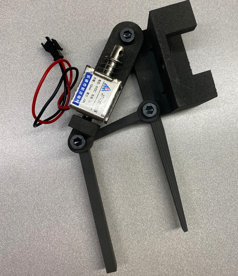
To design an end effector I took into consideration three factors: the force on the egg, compatibility of the design with the robot, and the total weight. Additionally, I was provided with geometric constrains shown below and the target range of 2 - 9 N exerted on the egg. The end effector is split into two components. The static (straight) component interfaces with the robotic arm with a dovetail. The dynamic (bent) component is moved by an actuator to grip the egg.

Dynamic Component

I landed on this final design after two rounds of design iteration. The greatest improvement during my design iteration process was adding an I-beam to each of the action arms. This improvement allowed me to improve the strength of the design while reducing the amount of material that was required.
In plain terms, an I beam works because it has most of its material far away from the neutral axis/center of the beam. Since that is where the strongest stresses will result during bending, this strengthens the beam making it robust under bending.
In engineering terms, an I beam works because it increases the moment of inertia by maximizing the amount of material away from the neutral axis. As shown, the moment of inertia for an I-beam will always be larger, leading to smaller deflection and therefore greater strength under bending.

Static Component

Physical Testing Setup

The stress analysis results (Von-Mises) were promising since the maximum stress predicted was around 6.04 MPa, well below the yield strength of Nylon-12.

Below I recorded the results of my real world testing and the FEA results. For both these experiments I forced a deflection to both 1mm and 2mm and then recorded the force required to reach this deflection on each element of the end effector. The setup for these tests can be seen below as well, with a force sensor attached to a moving arm.

Von Mises Stress Results from FEA

The end effector was able to pick up the egg and move it without cracking it!

The weight of the end effector, actuator and screws all together was 122 grams. This was 14 grams lighter compared to the first iteration, a difference due to reducing the material in my design and the screw size required to hold it together.

This final project for ME 240 was a fun application of the theoretical engineering topics that I have been learning up into my second year of college.